Chapter 2. The Democratic Classroom

This should not have happened! Today was the first day of third grade, and Janel was thrilled. In the democratic school that she goes to they let you choose which of the two third grade classrooms you will be in. You can choose if you will be in the classroom on the bottom floor that everyone calls DOWN, or the one on the second floor that everyone calls UP. Janel was very excited about this because she could be in the same class with all the kids she liked, like Olivia, Roger and Mia, but not be in the same class as Madison. Not only was she in the same classroom with her in second grade, but she even had to sit next to her.

Before I tell you more about what happened to Janel on the first day of school, I want to remind you that the fundamental concept I am exploring here is the notion that our social world is composed of frustrated systems. The world's real social systems are highly complex, but I will assume as a metaphor, very simple frustrated systems which can nevertheless generate significant complexity. Hopefully, some of the fundamental properties of these simple systems can be informative. I would like to stress again, I am exploring these systems not because they are a true model of the social world, rather they are a metaphor for some aspects of the social world, and hopefully insights gained from these metaphors will be informative.

So, let’s get back to Janel, and to her first day of third grade, a day that went so horribly wrong. Olivia lives just across the street from Janel, they are best friends and their parents were friendly. The parents decided that Olivia’s mom would walk both of the kids to school in the morning and that Janel’s dad will pick both of them up at the end of school. It’s hard to remember now, but the morning was a beautiful and exciting. When they walked to school with Olivia’s mom, the two girls chatted excitedly all the way, and then quickly ran into the school as they approached without saying goodbye to Olivia’s mom.

At the end of the day, when Janel’s dad picked the girls up, both girls entered the back seat of his car silently from separate doors and did not talk with each other. When Janel’s dad, asked them, as cheerfully as he could, how was your day, he got back mumbles that probably meant OK, though it was hard to be sure. The ride home was in complete silence. When he parked at home, Olivia left without saying a word and went straight across the street to her house. This was atypical because it was usually hard to keep the girls apart. Only when Janel and her dad entered their house did Janel mumble, “I hate Olivia, she is in the UP class with Roger, and I’m stuck in the DOWN class with Madison again. I don’t know why she did this to me”.

The decisions that Janel and Olivia, and yes also Roger, had to make in choosing their classroom are in some sense similar to the decisions that I had to make regarding SodaStream. When they choose which class to be in, in each classroom there were some kids they liked and others they didn’t. The decisions were not simple, or in other words, they were frustrating. In this chapter I will explore a very simple, that I call the democratic classroom, from it we might learn why Janel’s day went so badly. If we are lucky, we might also be able to generalize from this model to the more fundamental concepts we are playing with. Hopefully, we will learn a little about the process of choosing which sparkling water to drink, and maybe even solve all the problems of the world.

2.1 If the choice is ours, why are we still so frustrated?

To understand what happened between Janel and Olivia on the first day of school, we need to describe the rules governing how students choose a classroom in this democratic school. In this instance, on the first day of the school year 60 kids arrive at school. Since the class limit is 30 kids per class, this group must be split into two different classrooms. To presumably make the kids happier the school introduced a democratic process to let each kid decide which classroom to join. So how would such a process proceed?

Initially half of the students are randomly placed into each one of the two classes. Next, one student is randomly chosen, for example let’s assume Janel is chosen to be the one allowed to change classes if she wants. Janel then looks at the two lists and says: “well Olivia and Roger are with me in the UP class, and so are 11 more of my friends, but Madison is also in the UP class, on the other hand, the DOWN class has Mia, Jimi and Sarah, and 13 more of my friends. I have more friends in the DOWN class, and I can get away from Madison, so I want to switch”.

It might not be an easy decision for Janel because she really wants to be with Olivia, Roger and Olivia and her 11 other friends from the UP class as well, so it’s a little frustrating. She might also be happy to leave the UP class because Madison is there, and she really does not want to be in the same class as Madison.

According to the terminology of the last chapter, when Janel is in a different classroom than Olivia, and since there is a positive bond between them, this is a frustrated bond. Similarly, being in the same classroom as Madison is also a frustrated bond. If she is in a different classroom than Madison, this is not a frustrated bond. In choosing if to change classrooms, Janel used a decision strategy that minimized the number of frustrated bonds.

Janel hopes though that when she switches classrooms, some of her other friends will switch as well. She also hopes that maybe some of the kids she does not like in the new classroom, will decide to move to the other class, and be with Madison. She is expecting Olivia to follow her, because they really like to be together. This hope that her own decision will also affect the decision of other students might make sense. For example, Roger currently might have 15 friends in the UP class and 14 friends in the DOWN class, but once Janel moves, he will have only 14 friends in the UP class, and 15 friends in the DOWN class, so when it’s his turn to choose, he will likely also decide to switch to the DOWN class. However, note that by the time he gets to make his next decision, other kids might move between the classrooms, and the calculus might be different.

The main question we are interested in how Janel happiness or frustration levels change during this choice process. Will be happier, or less frustrated, in the classroom she ends up in at the end of this process than she was in her original randomly chosen classroom. We are not only interested in Janel though; we also care about Roger and even about Madison.

To better understand the process, I developed this simple Democratic Classroom game, that you can play. Playing the game can let you experience a similar situation and can also clarify some of the more formal concepts I will use below. When you start playing you will be prompted to enter your first name. Other student names will be chosen automatically. Initially students will be placed randomly into the two classrooms, the DOWN classroom (left) and the UP classroom (right). You will like about half of the other students, these students will have the same color box as you, students you dislike have a different color. Who you like and dislike is assigned randomly. Once you start the playing the game (green start button) one student will be randomly chosen at each time step, and they will be allowed to switch classes or stay in their current classroom. You will see the students names moving between the two classes. Your name will also be chosen at random, and then you will be allowed to make a choice as well. You will be able to shift between the UP and DOWN classrooms, by pressing the UP and DOWN buttons. The better choice, the one which will reduce your frustrations, will be marked in green. Below the classroom panel, you will see a panel with two curves, the blue curve shows how your level of frustration changes as the process evolves, the red curve shows the average frustration level of all the students.

As you can see when playing the game each iteration by a different student makes a choice. A student is randomly chosen from the group, and they can then decide whether to switch or not. This process is repeated until no one wants to change classes anymore. This repetition means that each student is likely to get several chances to choose whether to stay or move. Now, you might worry that this process will never end, and in general this is a possibility, but under some assumptions this process is guaranteed to end (Box 1).

What are these frustration curves though? Your frustration curve (blue) is formed by counting the number of frustrating placements at each iteration. By frustrated placements I mean, the number of students in your own class that you do not like + the number of students in the other class that you do like. The average frustration curve (red) is simply a curve of the average frustration level of all the students, at each iteration.

Note that if you make the preferred choice (green button) your frustration level will never increase due to this choice, but your frustration might increase when other students make their choices. For example, if Madison decides to move into Jannel’s class, Jannel’s frustration will increase. When you make the wrong decision (red button) you will often see your frustration level increase and it will never decrease. If you did not observe this yet, you can play the game again and deliberately make some wrong choices.

Note that if you make the preferred choice (green button) your frustration level will never increase due to this choice, but your frustration might increase when other students make their choices. For example, if Madison decides to move into Jannel’s class, Jannel’s frustration will increase. When you make the wrong decision (red button) you will often see your frustration level increase and it will never decrease. If you did not observe this yet, you can play the game again and deliberately make some wrong choices.

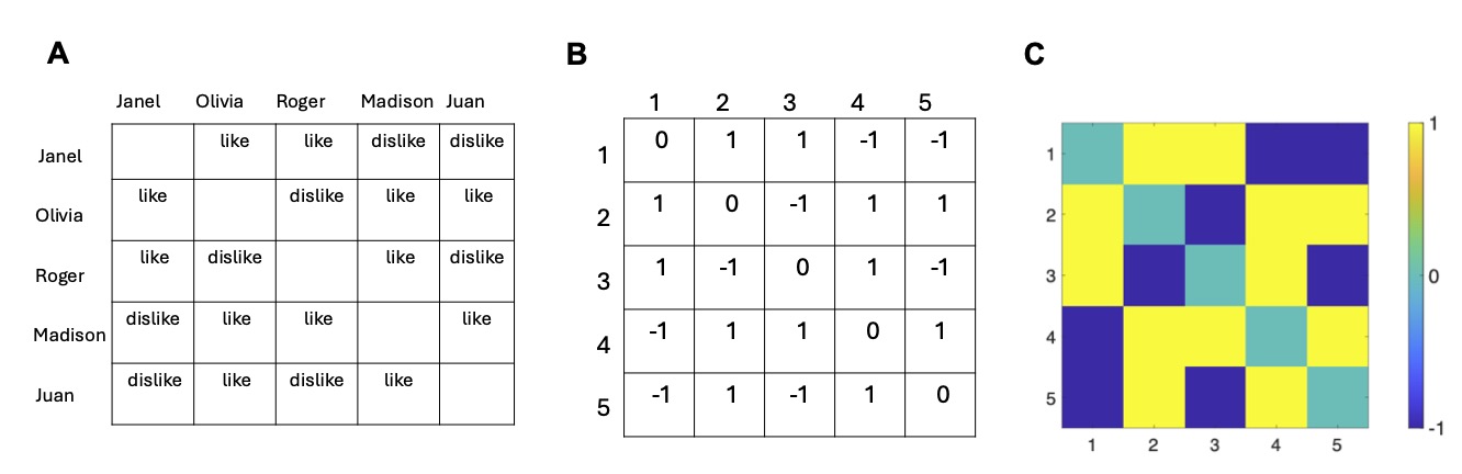
Even though you probably already played the game, I didn’t explain yet exactly how the game was constructed¹. Before each game is played, I determined who each student likes and dislikes. I assumed that each kid in class likes about half of the other kids, and dislikes the other half, l also assume that these affections are mutual (symmetric); that is, if I like you, you like me, and if I dislike you, you dislike me. Apart from this constraint, I assume that our liking preferences in terms of who we like, and dislike are assigned randomly. I also assume for simplicity that everyone we like, we like to the same degree, and the same holds for dislike (yes, I know). This process could be summarized in a table which lists which of the students, each of the other students likes, of dislikes. Figure 2.1A shows an example of such a table, for 5 students. To make representation more compact, I could replace the like by the number 1, and dislike by the number, -1. I could also replace the students names by a number. This representation is shown in Figure 2.1B. Such a representation is called a matrix in mathematics. We call this matrix here, the interaction matrix. To make this graphically more appealing we can color code this matrix - like is represented as yellow (like → 1 → yellow), and dislike as blue (dislike → -1 → blue), as shown in Figure 2.1C.

Initially, half the kids are placed randomly into one classroom, and the other half into the other classroom, this is the initial state. After the initial class placement, one kid is chosen randomly from one of the classrooms and they are allowed to make a choice. The decision rule is simple; the student chooses the classroom where they have a lower frustration level. The frustration level is defined as the number of enemies in the students current class and adding to it the number of friends in the other class, just like those depicted in the game. The student chooses the classroom where this number is lower. All other students always adhere to this decision rule, when your turn to choose you have the option to make the bad decision as well. The outcome of the decision rule is indicated by the red and green colors of the DOWN and UP buttons. You are the only student who is allowed to make the wrong choice. You should play the game and see how correct and incorrect choices affect your frustration level.

In figure 2.2 I show an example run of a democratic classroom simulation, similar to the one you just played, but using slightly different graphical representations. In this specific run, all students always made the preferred decisions. Figure 2.2A shows the interaction matrix. In Figure 2.2B I show a different representation of class placements in the initial and final state of the run. If a student is in the DOWN class they are represented by white, and in the UP class by black. Figure 2.2C shows how the class placement evolves over iterations, and Figure 2.2D shows how the average frustration index changes over the same process. The frustration index is simply the average frustration level divided by the number of students.

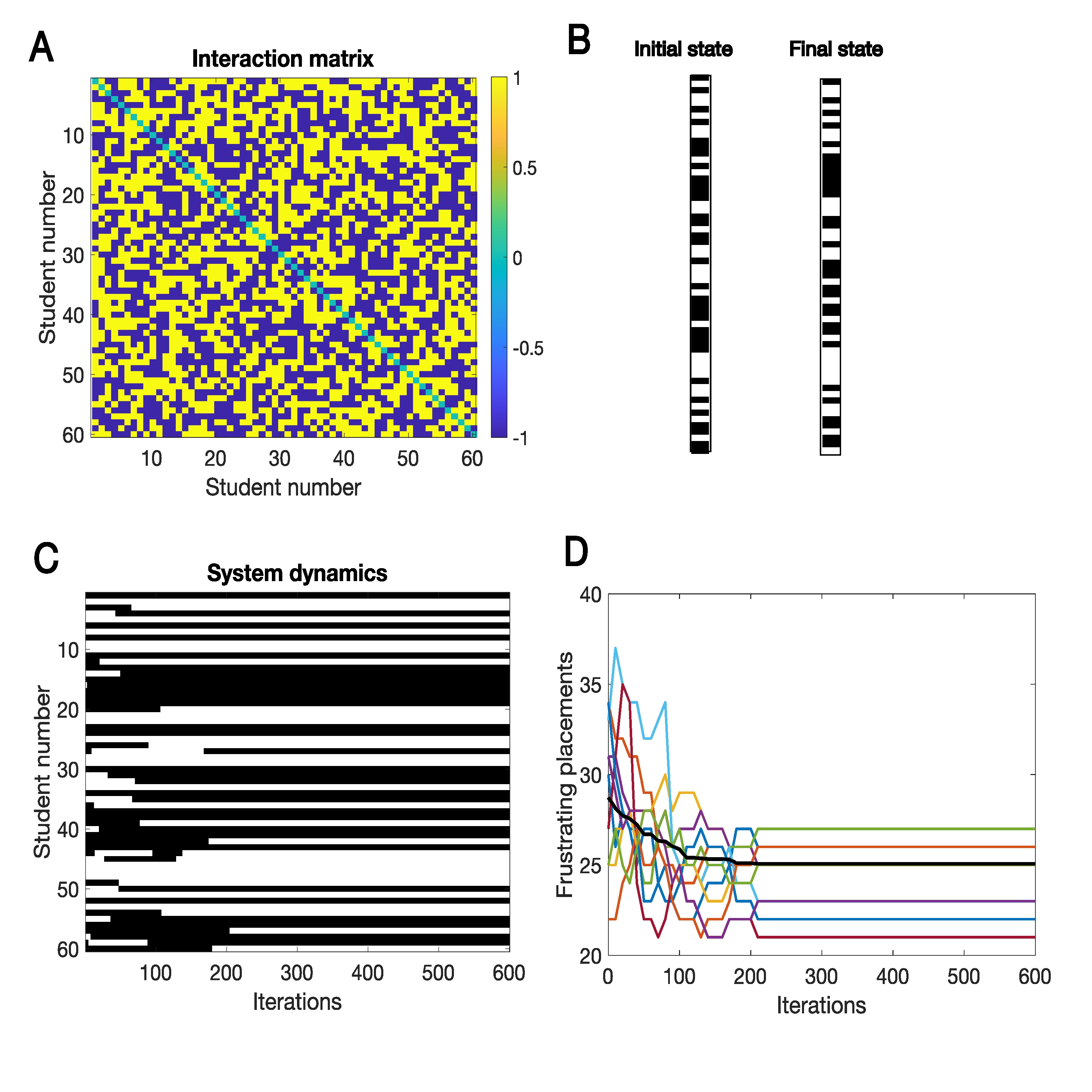
In Figure 2.2, we see that for this specific example that this choice process indeed ends. The class placements (Figure 2.2C) stop changing after about 300 time-steps. This is also reflected in the frustration index of Figure 2.2D which stops changing at the same time. The class placements do no change even though students are still allowed to change their preferred classroom. Students stop switching classrooms because they can no longer reduce their frustrations by moving. Intuitively one might wonder if this is the case in general or is it possible that this process will never stop. This is actually where intuition might be insufficient. Using mathematical methods, it is possible to prove, for this symmetric case (if I like you then you like me), that the process will end, and we will be able to start the school year. The mathematical proof, while not presented here in detail, is outlined in box 1.

One intuitive simple example to demonstrate that these decisions converge with a symmetric interaction but might not with an asymmetric interaction, is the case of only two students in two classrooms. If both students like each other, they will both end up in the same classroom and none of them would choose to switch, if both dislike each other, they will choose different classrooms. However, in the asymmetric case (I like you, but you do not like me), the class choice process can last forever.

In the following version of the game, you will be able to run exactly the same type of game as above but using the new representation of class placement. This is the same representation used in Figure 2.2. The advantage of this representation is that in one image we can see how the class placements changed throughout the process, whereas in the previous version we only saw the current state of the classrooms.

In the game shown in Figure 2.2 average frustration levels are reduced by this process but not eliminated (Fig. 2.2D). Any time you run this game you will see qualitatively similar average results. How is this reduction in average frustration achieved, do the frustration levels of all students decrease? Do some decrease by much, and others by a little? Is it possible that for some students the frustration levels actually increase? How can we assess this? One possible measure is to count for each of the students their individual frustration levels. This mean that for each student we count how many of the students in their own class they do not like and add to that the number of students in the other class that they do like (the number of frustrated bonds). For each student the level of frustration can change during this process. For example, Sarah might initially have 32 frustrating placements (or frustrated bonds), and at the end of the choice process only 25 frustrating placements. On the other hand, Janel might initially have 28 frustrating placements, but at the end have 29 frustrating placements.

We see that while choice reduces the average frustrations, it effects on individual students can differ. To understand more about the process quantitively we generate another type of a summary of frustrations across the whole population. This is done in the following manner. First, we calculate the number of frustrating placements for each student. Then we count how many students have zero frustrating placements, how many have one, and up to how many have 59. The results of the counting and binning process can be plotted in the form the bar plot, as shown in Figure 2.3A. The type of bar plot shown in Figure 2.3A is technically called a histogram. We plot these histograms both at the beginning (blue) and the end of the simulation (brown).

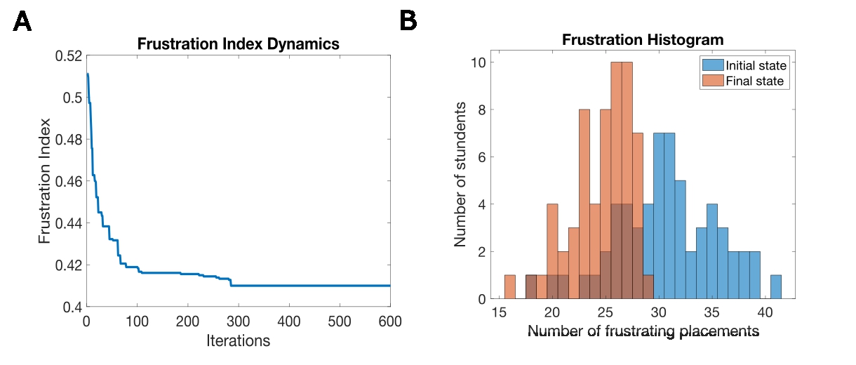
In the initial state (Figure 2.3B -blue) four students have 35 frustrating placements, but in the final state (brown) no students have more than 30 frustrating placements. In general, the frustration histogram in the final state (brown) shifts left when compared to the initial state (blue). However, the two histograms are overlapping. The shift implies that the choice process makes most students less frustrated. Since the shift is not huge and there is still an overlap it means that frustrations are reduced, but not by that much. Indeed, some students might actually become more frustrated by this choice process, such an occurrence is rare, but it might happen.

We might also want to examine how the frustrations evolve over time, but it is not easy to view the whole histogram for each time step of the choice process. In order to view how average frustrations evolve time, we examined previously the average frustration level, or the frustration index (Fig. 2.2D, Fig. 2.3BA). Initially as expected, the frustration index is approximately 0.5, and this choice process makes it smaller. Unfortunately, not by much. The initial frustration index is about 0.5, so each student on average is unhappy with about 50% of the students placed in their class, and the students placed in the other class. However, by averaging over the whole histogram, we do not see how this frustration is distributed across the population, as we can see from the histograms (Fig. 2.3A).

For this size of class, the final frustration index is about 0.4. This means the level of frustration was reduced by about 20% on average; it is better than in the initial state, but still not great. Under these assumptions, this system freezes, that is students no longer change their class preferences, and the frustration level does not change either².

Another interesting aspect is that although the system is egalitarian in its setup, in the final state some students are more frustrated than others (Figure 2.3A). While the happiest student in this simulation has only 15 frustrating placements, the unhappiest one has 29. This might be quite counter intuitive. Let’s assume for example that Roger is the student who has 29 frustrating placements, why will he not choose to change classes next time his name is called? The answer is simple, if he decides to switch, he will either be frustrated to the same extent or even more frustrated. If this were not the case, he would choose to make the change, and this will not be a steady final state.

One might ask then, what are the virtues of the happiest person which make them so happy? What are the annoying characteristics of the student who is significantly more frustrated? Or in the case of Roger we might ask, what is it about Roger that makes him so frustrated. We can use such a simulation, to investigate this question. In this case the happiest student was student number 28 (Jennifer). It turns out that if we run this simulation again, with the same interaction matrix (that is Janel still likes Roger and Olivia), but just starting with a different initial class choice, then the happiness or frustration of Jen or any other student will change completely and will be almost entirely unrelated to their happiness in this run.

To demonstrate the role of chance, I ran this simulation 3 more times, with the same interaction matrix, but with different initial conditions. I find that the frustration score for student who in the first simulation was the happiest (Jennifer, student # 28) were 27, 29 and 23, compared to 15 in the Initial run. Indeed, the final states of several runs, using the same interaction matrix, but starting from different initial conditions are very different and they seem almost totally unrelated. Though the details of these final states are different, on average the level of frustration is nearly identical.

These results mean that in general for such a system with exactly the same interaction structure, there are many approximately equivalent final states. This observation is actually a central point of this analysis. There is not one possible optimal world, instead there are many different configurations in which the average final frustration is very similar. What is different is which specific student is more, and which is less frustrated in each configuration. In this framework, the virtue which makes one person happier than the other is simply chance. Or to be specific Jennifer is happier than Roger because she happened to be luckier. I am not claiming here that this is the only virtue that matters in the real world. However, in a frustrated system the role of chance is inevitable.

In the real world though, Roger might truly be obnoxious, and that is why he is frustrated, or maybe why other people in his class are frustrated. In the very simple model system presented here we ignored this possibility, raising the reasonable objection that maybe luck is just an important determinant of fate in this simple model system, in which everyone was equally obnoxious, and that this observation has no bearing on the real world, in which some people are truly more obnoxious than others.

On a more general but technical note, these many possible final states imply that the energy function of this system (for example look at Figure 1.4B) has many equivalent minima. This large number of energy minima, or equivalently final states, is a hallmark of frustrated systems. These energy minima are closely related to the minima of the frustration index, which also has many nearly equivalent minima. In systems with frustrations there are in general many equivalent final states (or minima) each one with similar macroscopic statistics (e.g: average frustration, or frustration index). All of these final states are ‘better’ than the initial state, since the average level of frustration is lower. This improvement in frustration shows that letting students choose did make a positive difference. However, the frustration level in all of these final systems is not great, most students are still quite frustrated, despite their ability to choose.

In this exercise I created an egalitarian model world, in the sense that the number of friends and enemies of each student were almost the same. No student was significantly more popular or more hated than any other student. We initially placed students randomly in the ‘UP’ and ‘DOWN’ classes, and then let the students themselves choose which is the class they want to be in. When they made those choices most students became less frustrated, but not all, as seen by the overlap between the distributions of frustration initially and finally in Figure 2.1A. Although this ability to choose made more students less frustrated, some (tough not many) could actually stay just as frustrated in the process. Moreover, the final state is far from ideal for the average student, as the average frustration remained quite high.

This points to another problem with this egalitarian model world - it is just not fair! Some students remained quite frustrated, while others much less so. So, what are personality characteristics that made one student happier than another? It turns out that in this simple egalitarian model of a world, what makes one student happier and one more frustrated is simply luck.

2.2 Are bad decisions good for us?

Everything up to here assumed that each student always makes the decision that is ‘best’ for them, which is to maximize the number of friends and minimizing the number of enemies in their class. However, people sometimes do not make the ‘optimal’ decision. For example, if the students are tired, they might not count correctly or add correctly. They might also get tired of switching classes. Making such suboptimal but non-biased decisions is often called noise in the decision process.

Why do we call it noise? Think, for example, of listening to someone who is speaking softly. If you are listening to them in a quiet home, you are likely to understand everything they say, however if you happen to be in a noisy rock concert, or a noisy subway station, you might not understand correctly what they said. This noise affects how well we can read out the signal, in this example what the person is saying.

In simulations we often add ‘noise’ by simply adding or subtracting a random number obtained from a random number generator. So, for example, if the correct count is that in my current class, I have 2 more friends than enemies. When adding noise, we might randomly add to 2, a random number in a given range, say from -3 to +3. If this random number is large enough, it might affect our decision by making us mistakenly think we have more enemies than friends. On average this type of noise will not change the direction of the decision in a consistent manner since the mean of this random number is zero. This means the noise is not biased but can still cause us to make the wrong choice.

If the range of these random numbers were small, say -1 to +1 this will not make a big difference to decisions, if it is large, it might swamp the actual count. The more noise there is, the more often each student will fail to make the optimal decision. In this section we ask the question, how bad is noise, or might some noise even be good in some sense. In Box 2 I explain mathematically how noise was added here. In physics such noise is actually related to temperature; high temperature means high noise. In box 2 we also intuitively explain how temperature and noise are related.

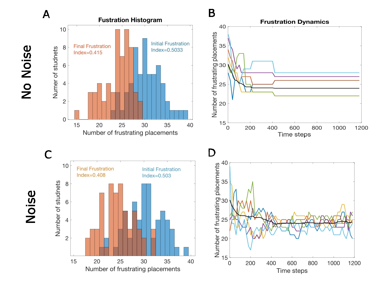
We simulated class choice both when students make optimal decisions, and when they do not. Or in other words, both with and without noise. The comparison is shown in Figure 2.3, where on the top panels (Fig. 2.4A,B) we see noise-free simulations and on the bottom panels we see results of simulations with moderate noise (Fig 2.4C,D). These simulations show us that the final distributions of frustration with and without noise are quite similar (Compare 2.4A to 2.4C). So, at the level of the population, bad decisions do not make things significantly worse, or maybe not even worse at all. In the simulation with noise, you sometimes see small transient increases in the frustration level (Fig. 2.4D, black line). Nevertheless, the average final frustration index is also quite similar, 0.415 without noise and 0.408 with noise, for this specific simulation. When this type of simulation is run many times no significant difference is observed in terms of the final mean frustration index. We can conclude that noise at this level, made little difference on to the average level of frustration.

What is very different though is what happens to each individual person over time. This is seen by comparing the colored lines in Figure 2.4B and 2.4D. These lines are the frustration levels of several randomly chosen individuals. In the ‘noise’ free case (Fig. 2.4B), these frustrations quickly reach their final level, or in other words they freeze. On the other hand, when noise is added, these individual plots keep changing (Fig. 2.4D), even though their average is highly stable.

What this means in the specific example given above is that without noise Roger remains unhappy throughout the process. In general, specific people rapidly become less or more frustrated, those who are more frustrated, remain so, and those who are less frustrated also remain less frustrated. The initial luck, which made some happier and others less happy sticks. On the other hand, when people sometimes make bad decisions the system remains fluid, people who were initially more frustrated become less so, and the less frustrated students become more frustrated, and this constantly changes over time. In Roger’s case, although he was initially highly frustrated, over time he became less frustrated, and maybe later more frustrated again. So why will Roger’s ability to make bad decisions make him happier? It turns out that it is not Roger’s bad decisions that make him happier, instead Jenifer’s and Omar’s (sorry, I forgot to mention Omar earlier) bad decisions, which make Roger happier. Jennifer and Omar were initially quite happy, however because they sometimes make bad decisions, their initial luck does not stick, and they might become more frustrated over time. This makes the system more dynamic and allows Roger to become happier over time. In general, the bad decisions by the initially lucky students allow the less lucky students to become happier, for a while. This might be confusing, since on the global level the average level of frustration does not change for a moderate level of noise, yet the frustration of each student is very different in both cases. What this means is that the single measure of average frustration does not tell everything about the system – for example it does not tell us if the system is frozen or mobile.

I think this needs to be clarified further. The kids who become happier due to noise, are not happier because they directly enjoy the misfortune of those who made mistakes, they actually become less frustrated themselves. How does this happen? For example, lets assume Madison erroneously leaves her current class. This might directly make Janel, happier. On average though it will not make the class happier, because Madison has many friends in her current class, who will be sad to let he go. If you look carefully at the black line of Figure 2.4D you will see average frustration occasionally increasing, something that never happens in the noiseless case. However, after Janel’s mistake, the next person who chooses, might now see that it is now advantageous for them to switch classes. This ability to become less frustrated by switching classes was made possible by Madison’s mistake. Without noise, the class structure freezes, as is evident in Figure 2.4B where no more changes occur after about 400 iterations. No changes occur, because no one can gain from changing, even if they are highly frustrated. On the other hand, once noise is added, the class structure is thawed. This does not make the class of average happier. Indeed, for a larger amount of noise the average frustration would increse. What adding noise does is that across time, who is specifically more or less frustrated changes.

If we raise the noise level further the noise will swamp the signal. In this high-noise case the histograms will no longer shift to the left and the frustration index no longer systematically decreases, instead it fluctuates around 0.5. In other words, when the information conveyed by the signal is lost in the noise, democracy is useless.

So, are bad decisions good for us? My bad decisions are not good for me, but they might be good for other people, at my expense. For society as a whole are bad decisions good? That of course depends on your point of view. Some of the students in the class (Jennifer for example) might compare the messy dynamics of Figure 2.4D to the more ordered dynamics of Figure 2.4B and say: “what is the world coming to?”. Some students might think that the world with noise is unnerving, constantly changing and people don’t know their proper place anymore. Others, however, might welcome this more messy and more dynamic world. Each student’s points of view on the issue of whether bad decisions are good, might depend on their personality, but is likely to also depend on where they personally fell within the initial distribution of frustration.

2.3 Other frustrating games

While Janel and Olivia indeed had a difficult start of the school year, Brian a resident of Santa Fe, New Mexico had a hard decision to make each evening. Brian’s favorite bar in Santa Fe is the El Farol bar2. It is his favorite activity in the New Mexico summer evenings, but ithe bar is small. If more than 60 people attend the bar it is quite miserable. The problem is that on most evenings up to 100 people may want to go to the bar. Brian has a problem, if less than 60 people go, he will prefer to go to the bar than stay at home, but if more go, he will rather stay at home. There is no way for Brian to know how many people will actually show up on a given night.

The El Farol bar problem was introduced by economist Brian Arthur to illustrate a problem with the typical approach of economists, an approach that depends on inductive reasoning. This problem was later mathematically analyzed by physicists and mathematicians who had shown that in this problem is analogous to a frustrated system, or a spin glass system2. Each potential customer of the bar has opposing forces, on one hand they would like to go, which is similar to a positive bond, but on the other hand they fear that too many other people would go as well, which is analogous to a negative bond. Like in the democratic classroom game, not everyone can be happy, because if 100 people go to the bar they will all be unhappy, but if only 60 go then 40 would be frustrated. The El Farol bar problem is an example of a wide set of problems called Minority Games². Also, if the ideal solution is that only 60 people go to the bar, there is a question of which specific other people would go. In other words, like in other frustrated systems, there are many equivalent solutions that minimize but do not eliminate frustrations.

Brians problem is whether to go to the bar of not, but Merril and Melvin have a bigger problem, how to minimize the time they will spend in prison. Police investigators suspect them of a robbery, but do not have enough information to convict them of that crime. If they are convicted of robbery without admitting, they will get a 4-year sentence. Without additional evidence they can be convicted on the smaller offence of holding stolen property for which they will only serve one year in. The suspects are put into separate rooms and are not allowed to coordinate. The investigators tell each one of them separately, that if they betray their accomplice and testify against them in court, they will go free. If both betray, they will each get a 3-year sentence. On average the best decision for them is not to admit, but they both fear that the other one will betray them, and both are tempted by their potential to go free without spending any time in prison. This hypothetical game, called the prisoners dilemma, is the most famous game in the field of game theory³. Its attraction stems from the conflict between what is the best decision for each of them, and what decisions minimize the total time they will spend in prison.

Game theory is in general a mathematical field that tries to actually address not the games people play, but instead economic and social interactions between people3. Interesting games have conflicts and are supposed to be simple models of the conflicts in real life. Complex games, that is games which have many players, and many strategies can be quite similar to frustrated systems and the democratic classroom². They too have solution that can reduce but not eliminate frustrations. They have many equivalent solutions with similar levels of frustration but in which the level of frustration of each agent is different.

The aim of this short section is not to explain complex systems in economics or to explain game theory. There are many excellent sources both popular and professional addressing these fields^2,3. The aim of this section is to clarify that other models of complex social systems have been proposed over the years. Under some conditions those systems are similar to the frustrated systems described in in this project.

2.4 So what does this all mean, if anything?

So, what did I claim and show up to here?

1. Many decisions in the social world are frustrating in that there are no options which satisfy all constraints, in which we achieve all that we hoped for. Additionally, our own decisions have an impact on the well-being of others and on their decisions as well. This makes our social world a frustrated system.
2. Frustrated systems have many equivalent outcomes. This might possibly be non-intuitive, at least to some of us. There is no one best solution, there are many solutions that are on average similar. This is analogous to what in the physics language is called many local minima.
3. History is not inevitable. For exactly the same system, with exactly the same interactions, the final outcome can be quite different depending on the random initial condition and on noise. This means that the present state was not inevitable, history could have taken many different turns, even in such a simple system. The frustration index for all of these different final states is similar, but the identity of who is frustrated and who is happy changes.
4. The dynamical process in which each person makes the best choice for them reduces frustration, yet each person remains quite frustrated. In the final state some are less frustrated than others, but where each person ends up is fully determined by chance, or in other words by luck.
5. In a noise free system, in which everyone makes the optimal decision, the dynamics quickly freeze, that is there is no more mobility. Those who were less frustrated, due to good luck, remain less frustrated, and those who are more frustrated remain screwed.
6. Bad decisions, or noise, unfreeze the system. The levels of average frustration do not change much, but mobility is reestablished. In such a noisy system, although the average level of frustration is similar to the noiseless system, each person goes through phases where they are more frustrated or less frustrated, and over time the average frustration of each student is similar to the average frustration of the whole population.
7. If the noise is very large, choice and the democratic process is useless.

A note of caution. Although I use mathematical models to make these statements, I am not claiming that any of the quantitative results these models generate are precise predictions about the world. Instead, I use these very simple models as metaphors of the world. Therefore, my statements, even though the Figures I show below have numbers on them, are qualitative in nature.

Yes, I know, I didn’t explain yet which type of Soda is best for the world, and also, I didn’t explain what exactly is wrong with Madison.

2.5 But, but, but, but

So, when my wife read a draft of this chapter (without this section) she said: but, but, but, but. To be more precise (and I am paraphrasing what she is saying because I don’t record everything we say at home), she said:

• but kids don’t really care about all other kids in class, they like some, might dislike others but they are neutral about most. Really, mostly, they want a few friends
• but some of the other kids that I liked, I might like a lot and others a little, and the same holds for dislike. This is not included in your assumptions.
• but some of the other kids one dislikes at the beginning of the school year might become their friends after a few weeks or months.
• but some might choose to stay in the same class after a while, even if switching is better, because they might become tired of switching classes.

All of these objections make sense, and there are many more.

So, with so many mistakes at the outset, could this model tell us anything about a real classroom?

My answer is yes; it may still be informative. This model might not be a very precise model of a classroom, but it can provide us with intuition about the world in general. An answer that to many of you might not make sense. The type of thinking I am using here is rooted in the style of thinking of physicists, it both motivates how we explore a problem and is motivated by previous results. This subsection briefly tries to explain this mode of thinking.

Before explaining this approach used by physicists though, I must comment that it is not only physicists who use such an approach that we can capture the truth by using imprecise assumptions. Authors of fiction can be much more blatant in this respect. For example, consider the quote: “Fiction is the great lie that tells the truth”, writes Abraham Verghese in the content of water⁴.

So, if we are talking about fiction let’s describe what really happened with Galileo and the Tower of Pizza⁵. Myth is that Galileo went up to the tower with two objects of different weights, that he dropped them simultaneously, and that they landed on the ground at the same time. This experiment is thought to be the basis of modern physics. In “truth”⁵ it was not really Galileo but his assistant Simplicio who at some point in the 16’th century climbed up the Pizza tower and dropped two objects at a time, to see which one fell faster3. He repeated this many times with different pairs of objects. Below we see a partial table he compiled of the objects dropped.

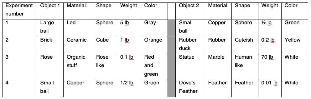
After 4 of these experiments Simplicio becomes tired of walking up and down the stairs. Actually, in the 4’th experiment he simply used a dove’s feather he found at the top of the tower, and the same ball from experiment 1. By now, if we have taken Physics in school, we also know what the answer should be. We would expect to hear Simplicio say “All these fucking objects reach the ground at exactly the same time, it does not matter if they are red or green, made of metal, marble or feather, their shape does not matter either, and even their weight does not matter, can we stop doing this boring experiment already, or if we have to keep doing it can we install an elevator?”

In reality, though this is not what Simplicio (had he existed) would have observed. In general, the lighter objects would have taken more time to fall. In reality, even two identical light feathers would have taken a different time to reach the earth. Galileo’s thought experiments and Newton’s mechanics which follow them assume a lack of friction, and in that simplified world indeed all these objects would fall at exactly the same time. Science, and abstract thought in general require such simplifying assumptions.

Note however, that if we ignore friction, we would not be able to correctly calculate how long it would take for objects to fall. In some cases, even with the most modern mathematical methods it would be hard for us to predict exactly how long it would take for some objects to fall, for example in the case of the feathers. We ignore friction here to obtain a simple abstract understanding, and later we can add more complexity to obtain an even better agreement with reality. These thought experiments, and these abstractions are essential for any form of abstract thinking, and here I am trying to follow this tradition.

It is not that it does not matter in general if the rose is red, or if the rubber ducky is yellow. But it does not matter for how fast they fall. It might matter in general if the rubber ducky is made of rubber and not led. For example, rubber duckies made of led are not likely to float well in a bathtub. Similarly, all the other details in the table above might matter in general, but not for how fast these objects fall in vacuum. Even though we do not live in a vacuum, assuming a vacuum makes it possible to generate a simpler understanding of the world, which can then be elaborated for the understanding of physics in those unfortunate planets that have an atmosphere.

OK, so my wife had problems with my simple, possibly simplistic model, and in response I make up a story about Galileo? Does that seem convincing to you? How are these things related?

The answer is that in Physics we have concluded that most real-world systems are too complex and difficult to solve exactly while incorporating all the details. At the same time, we have also concluded that many of these details may not matter, at least for specific questions. Instead, the notion of a universality class was introduced. One can see that many different systems, in which the details of interactions between the different elements are quite different, still behave in very similar ways. All of these systems belong to a single universality class, and only a small number of details about the interactions, or about the geometry of these systems seem to matter. Other systems might have different behavior, but these too can be grouped into other universality classes. In a sense what I am proposing here is that the social world can be understood as belonging to a class of frustrated systems. Though the details of these systems do matter for many of these systems properties. Other very general properties, like those listed in the previous section, are universal. My aim here is to use the physicists type of approach for gaining into social systems, and this included the use of simplified model systems (toy models) which hopefully capture some essential features of the social world.

Endnotes: Chapter 2

1. This game is very similar to the Sherrington-Kirkpatrick (1975) model. (Solvable Model of Spin-Glass, Physical Review Letters, 35:1782, 1975). The paper is included in the book: Spin Glass Theory and Beyond by Mezard, Parisi and Virasoro (1987). This paper, as made clear by its title, and most other papers in the book are mostly concerned with developing the statistical physics techniques necessary for solving such models. Solving means being able to state in a definitive, mathematically justified ways, how such models behave. In physical terms these models deal with phase transitions, and how these possible phases depend on the system parameters, for example the interaction matrix and the temperature (noise). While these mathematical techniques are beyond the scope of this book, the conclusions drawn in this chapter, as summarized in section 2.4 are determined by the results of these techniques.
2. The El Farol bar problem was conceived by Brian Arthur in 1994 in the paper Inductive reasoning and bounded rationality (The American economic review, 84(2):406–411, 1994). It is discussed in the context of the more general problem of Minority Games in the book chapter: Applications of spin glass idea in social sciences, economics and finance. (JP Bouchaurd, M. Marsili and JP Nadal, in the book: “Spin glass theory and far beyond,” 2025).
3. Game theory developed starting in the 1920’s, is a mathematical theory that analyses strategic interactions between people, entities or even countries. A major force in developing game theory is the renowned mathematician, John von Neumann. The book “Prisoners Dilemma” by William Poundestone, is an easy-to-read biography on von Neumann’s life, the book also explains in an easy to understandable way elements of game theory. There are many academic books on the topic, for example: Game Theory: an introduction by Steven Tadelis. The prisoners dilemma itself was conceived by Merril Flood and Melvin Dresher, at the RAND corporation in the 1950’s. The RAND corporation was the center of research in the field.
4. Abraham Verghese- The covenant of water (2023).
5. Obviously, this story I tell about Galileo is a fabrication. Simplicio though was a character invented by Gelileo and used in his book Dialogues on Two New Sciences (1638). Since Galileo has not employed him for hundreds of years, I took the liberty to use him for my purposes. What really happened with Galileo in the tower pf Piza is not known. However, it seems that other Similar experiments had been conducted in Delft by Stevin and de Groot. A popular article describes that describes this was published by Alexandra de Castro in 2021 in the United Academics Magazine. What is clear though, that no experiment conducted during those years could have resulted in the idealized result that a feather and a led weight would drop at the same rate.

Back to table of content

Chapter 3